Dóra Gavló

In the second part of the series we are going to look at the Expanding Polytope Algorithm, or EPA. EPA can give us the contact normal, penetration depth and 1 contact point per frame

Overview

1. Introduction
2. Terminology and recap
3. The Algorithm:
   
   1. 2D
   2. 3D
4. Contact point generation
5. References & the complete code

Introduction

So what is EPA?

The algorithm was created to calculate the penetration depth of two colliding objects. It does so using the results from GJK, which only tells you whether or not two shapes are colliding.

Advantages and disadvantages

Pros	Cons
Fast to implement	Can only give 1 contact point per frame
Works with any convex shape.	Complex shapes can significantly slow it down.

Terminology

Minkowski sum and difference

Both in GJK and EPA we work with points on the edge of the Minkowski difference. The simple definition of it is "subtracting all points of object B from all points of object A". This does not refer to all vertices but the infinite amount of points on each object. When the objects collide, the Minkowski difference contains the origin, which means they have at least one mutual point. This is because: (x1, y1, z1) - (x2, y2, z2) = (0, 0, 0).

Sometimes you might see this referred to as the CSO, or Configuration Space Object.

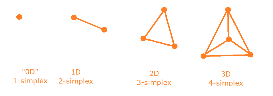
Simplex

This is the result from GJK and will be our starting polytope. In short, a simplex is lowest amount of points that are needed to define a shape in a given dimension.

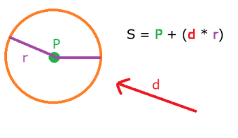
Support functions

Once again we'll rely on support functions to expand our shape. These give us "the farthest point on the object in a given direction". We will use this to get new points on the edge Minkowski difference and therefore extend our simplex. What shapes your algorithm works with depends on what support functions you write.
Below are two of the simplest shapes, but refer to the end of the GJK post for more examples.

GJK recap

Before we start with the algorithm let's quickly step one of our collision detection system in 3 points:

• GJK is a very fast algorithm that can tell us whether or not there is a collision between two convex objects
• It does so, by iteratively adding and removing points from a simplex, trying to create one that encloses the origin.
• If it manages to build a tetrahedron (or triangle, if we're working in 3D) that encloses the origin, we have a collision.

The algorithm

The goal of EPA

We're going to break the algorithm down to two parts. First, we'll get the penetration depth and the contact normal, then take a look at contact point generation. As I mentioned before, our starting polytope is the simplex from GJK. A polytope is a shape with flat sides, however thanks to support functions our algorithm can handle curved shapes, such as spheres too.

Our goal in the first step is to find the feature on the Minkowski difference that is closest to the origin. A feature is a line or a plane, depending on what dimension we're working in.

The core concept

Before we go into specifics and start coding let's look at what EPA actually does.

1. Take the simplex from GJK and "convert" it into a polytope
   
2. Calculate the normal and distance from the origin of every feature
   
3. Select the feature with the smallest distance
   
4. Get a support point in the direction of the feature's normal
   
5. Is the new support point further than the smallest distance in our current polytope?
   • Yes: add the point to the polytope and go back to step 2
     
   • No: we have found the closest feature. This feature's distance from the origin is our penetration depth and its normal is the contact normal.
     

2D

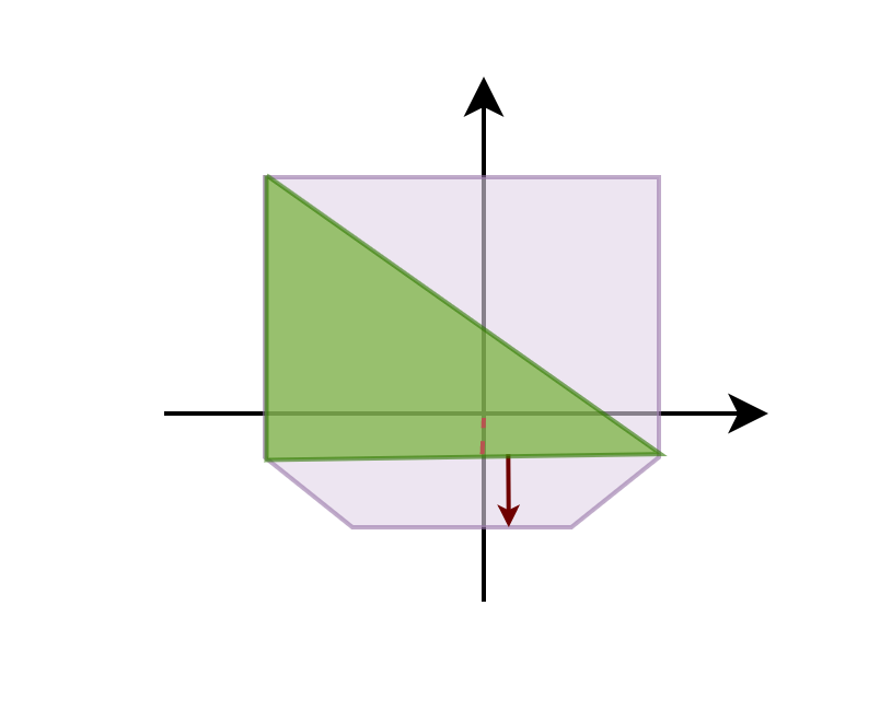
In 2D we start with a triangle simplex with the feature being the edge. Let's look at how the theory translates to 2 dimensions!

Converting the data received
You may recall from GJK that we calculate the normal of an edge/line with the triple product. We're going to use this method here too.

What exactly is the triple product?
We know from basic vector math that the cross product, denoted with x gives us a vector that is peprendicular to the input vectors. Crossing the resulting vector with one of the input vectors gives us one that is perpendicular to the input vector. However in this case there can be issues.

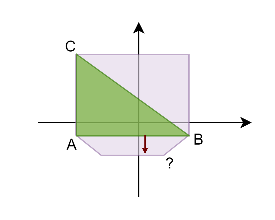
If the edge we are looking at is very close to the origin we can end up with a zero vector when calculating the triple product. Fortunately in 2D we have another way to get the edge's normal: simply flipping the components!

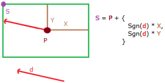
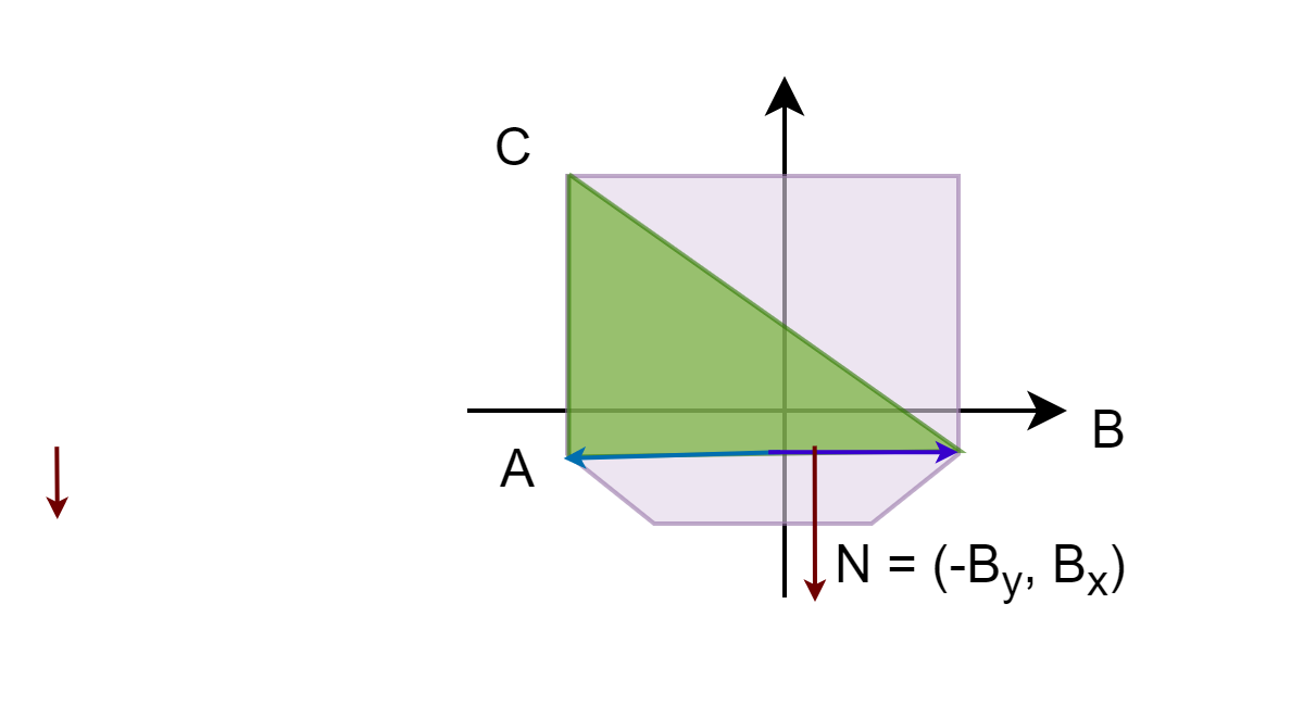
Flipping components and winding

When using this method we need to make sure that we use the correct winding. Winding can be clockwise (CW) or counter-clockwise (CCW). This defines which of the two components you need to flip. As an example, in the picture below we have the coordinates CCW order so we use the components of B.

Finding the closest edge

In 2D we do not have to store the edges as the calculations are relatively cheap. Once we have the edge's normal (either by the triple product or flipping the components), we can calculate the distance with the dot product. This is called projecting the edge onto the origin. Do this for every edge and you found the one closest to the origin.

	CEdge closest = CEdge();
	closest.m_Distance = std::numeric_limits::max();
	for (int i = 0; i < a_Polytope.size(); i++) {
		int j = 0;
		if (i == a_Polytope.size() - 1) { j = i + 1; }

		CVector2 a = a_Polytope[i];
		CVector2 b = a_Polytope[j];

		CVector2 edge = b - a; 
		CVector2 oa = a; 
		 CVector2 normal = TripleCross(edge, a, edge);
		normal.Normalize();
		
		double distance = ((a + b + c) / 3).Length();
		
		if (distance < closest.m_Distance) {
			
			closest.m_Distance = d;
			closest.m_Normal = n;
			closest.m_Index = j;
		}
	}
	return closest;

The main algorithm
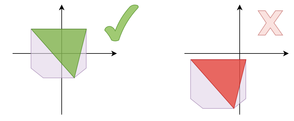
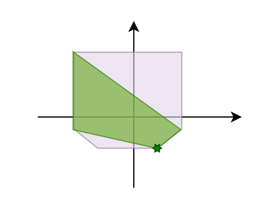
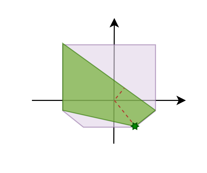
The 2D version mostly goes as the core concept above shows with no caveats. When we add a new point we can be sure that it'll be "between" the points that define the edge. Therefore, when we expand the polytope, the new coordinate needs to be inserted between the aforementioned two points. This also means that the list of points has preserved the winding order.

Finally, let's look at it in code

std::vector polytope = { a_Simplex[0], a_Simplex[1], a_Simplex[2] };
while (true) {

	CEdge e = ClosestEdge(polytope);
	
	CVector2 p = (A->GetCollisionShape().Support(e.m_Normal) + A->GetOrigin()) -
		(B->GetCollisionShape().Support(-e.m_Normal) + B->GetOrigin());
	// check the distance from the origin to the edge against the
	// distance p is along e.normal
	double d = p.Dot(e.m_Normal);
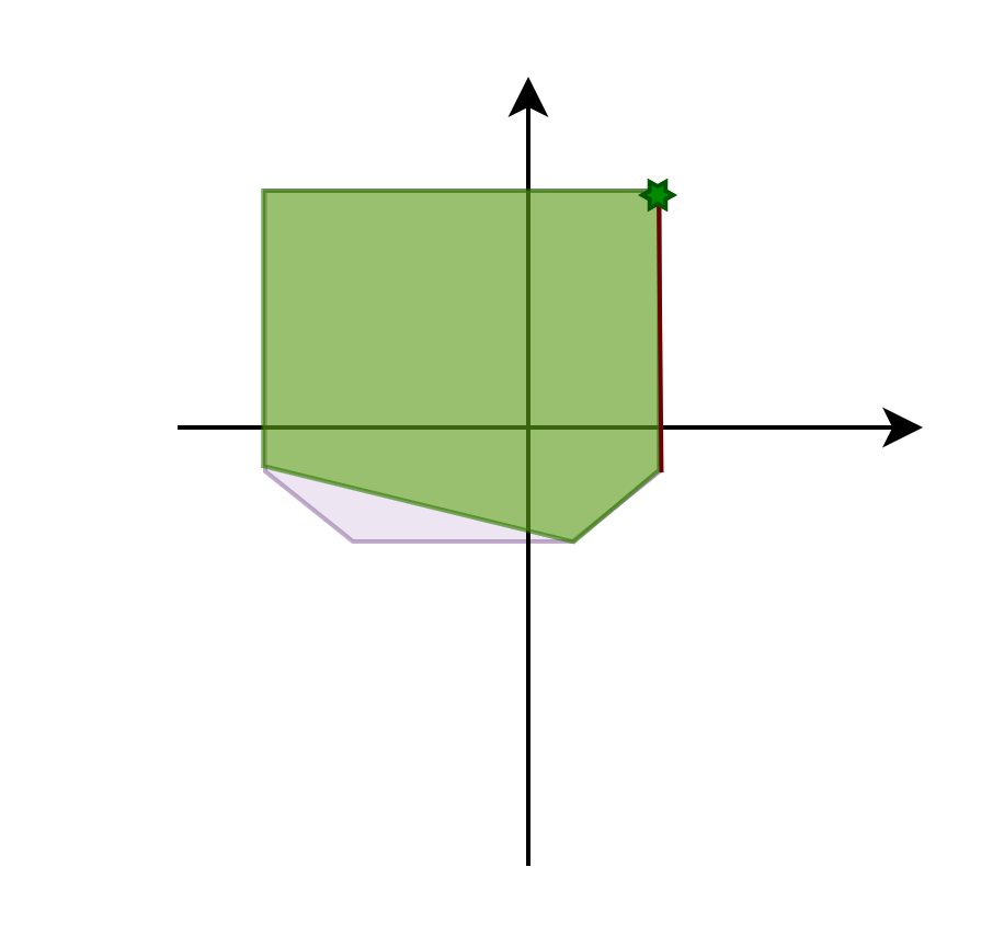
	if (d - e.m_Distance < 0.00001) {
		collision_normal = e.m_Normal;
		penetration_depth = d;
		break;
	}
	else {
		auto it = polytope.begin() + e.m_Index;
		polytope.insert(it, p);
	}
}

And that's it for 2D! Now let's add another dimension, which is where our issues start.

3D

In 3D, we start with a tetrahedron with its faces serving as features, which are triangles. Similarly, we use the triple product to calculate the normals. Unfortunately this time we cannot simply flip components anymore.

Issues in 3D
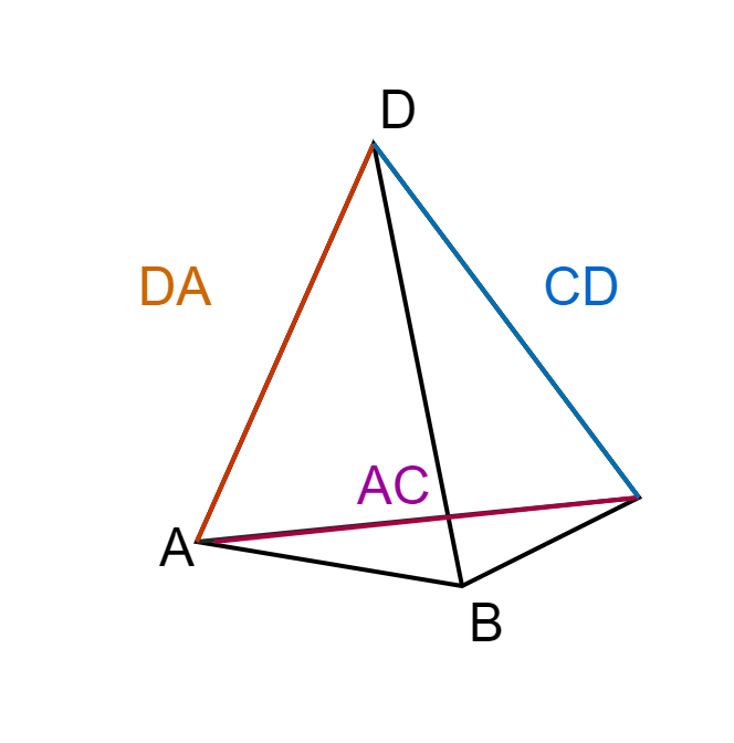
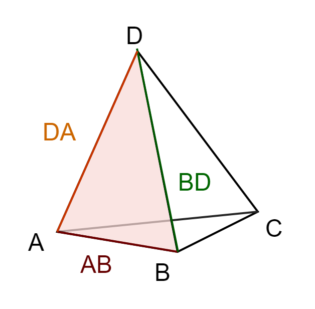
When adding a new point in 3D, you're creating new faces. The new face(s) contain 3 points: the newly found support point and the two ends of the "nearby" edges. However, when looking at the existing edges you might find some that are in the list twice. This causes problems as you could add the same face twice. To avoid this, we need to cull the duplicate edges. We'll look at this in more detail in a bit, but let's start from the beginning of the algorithm.

Converting data received from GJK
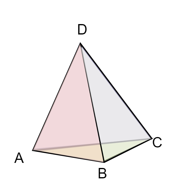
GJK algorithm yielded us a tetrahedron consisting of four points. In 2D, we could easily combine any two points to form a simplex feature, but in 3D, we need to do some calculations to determine the simplex's faces. Let's delve into this in more detail.
We know how the indices are ordered in the simplex, so we can simply hardcode it.

std::vector polytope = { a_Simplex[0],a_Simplex[1],a_Simplex[2],a_Simplex[3] };
std::vector faces{
0,1,2,
0,3,1,
0,2,3,
1,3,2
};

std::pair, size_t> temp = CreateNormals(polytope, faces);

In addition to the vertices, the normal and distance of the triangle from the origin are also necessary. To obtain the normal, we can use the cross product which yields a vector perpendicular to the two input vectors. In this scenario, the input vectors represent the sides of the triangle: B - A and C - A. By projecting the triangle onto the origin, we can determine its distance.
Once we have these values, we select the face that is currently closest to the origin and start our calculations.

std::vector face_data;
unsigned int min_triangle = 0;
CScalar min_distance = std::numeric_limits::max();
for (unsigned i = 0; i < a_Faces.size(); i += 3)
{
CVector3 a = a_Polytope[a_Faces[i]];
CVector3 b = a_Polytope[a_Faces[1 + i]];
CVector3 c = a_Polytope[a_Faces[2 + i]];

CVector3 normal = CVector3((b - a).Cross(c - a));
normal.Normalize();
CScalar distance = ((a + b + c) / 3).Length();
if (distance < 0)
{
normal *= -1;
distance *= -1;
}
face_data.emplace_back(CFaceData(normal, distance));

if (distance < min_distance)
{
min_triangle = i / 3;
min_distance = distance;
}
}
return std::pair, size_t>(face_data, min_triangle);

Note: in other tutorials/examples you may see the distance being calculated with Normal.Dot(A). This is a nice trick to speed up the algorithm, however it can give incorrect results when the projected origin on the triangle's plane does not actually overlap with the triangle.

Expanding the polytope and when to stop
The basic structure of the algorithm is the same as 2D: we use the normal of the smallest feature as our search direction. Every round we're creating faces on the edge of the Minkowski difference that are closer and closer to the orign. At some point we end up not managing to get any closer to the origin than in the previous step. That is when the algorithm terminates.

while (go)
{
min_normal = face_data[min_face].m_Normal;
min_distance = face_data[min_face].m_Distance;
go = false;
CVector3 A = a_Contact->m_First->GetCollisionShape()->Support(min_normal)
+ a_Contact->m_First->GetTransform().getOrigin();
CVector3 B = a_Contact->m_Second->GetCollisionShape()->Support(min_normal * (-1)) + 
				a_Contact->m_Second->GetTransform().getOrigin();
CVector3 support = A - B;
CScalar distance = min_normal.Dot(support);

if (CUtils::Abs(distance - min_distance) > 0.001f)
{
	go = true;

	//repairing code goes here…
	polytope.push_back(support);
	
   }
   else { go = false; }
}

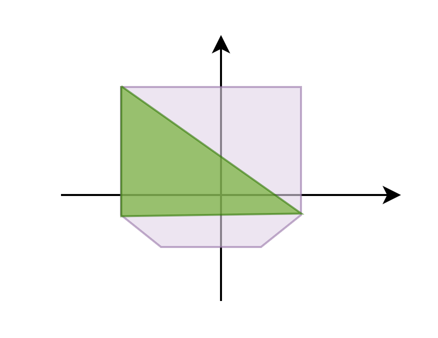
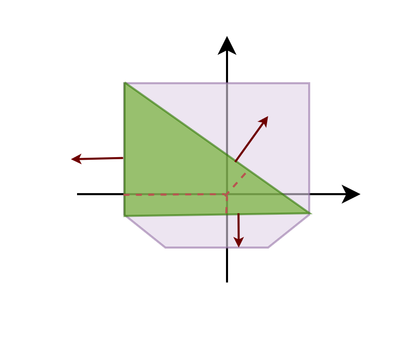
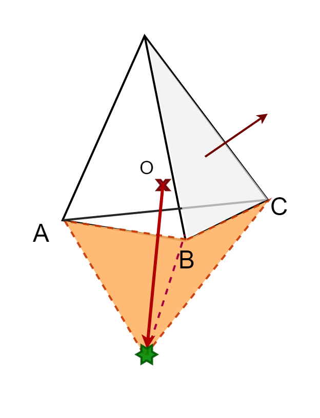
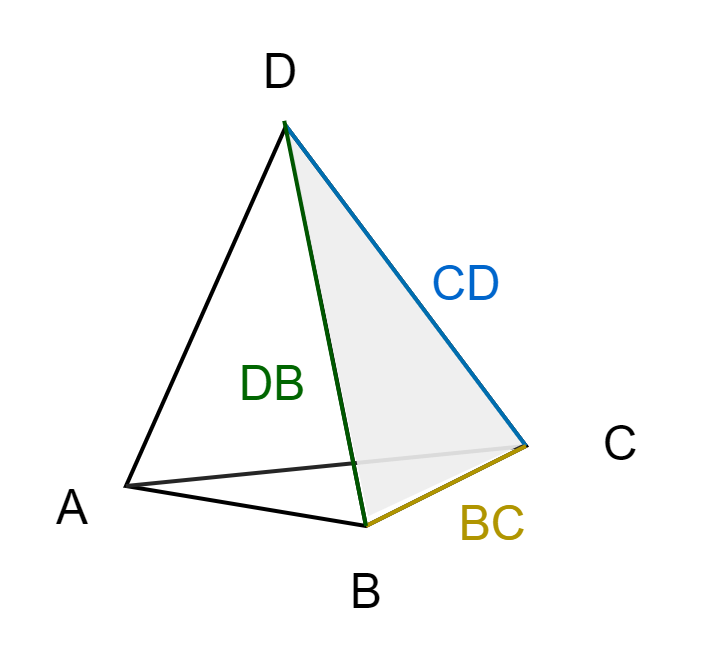
Finding the edges to connect to
In 2D we had a rather simple life since as we only had to insert a point between the edge that was our search direction. In 3D, adding one point can create any number of new faces. Therefore, we'll need another way to determine which faces to remove and which edges will help build the new faces. You may recall from GJK that testing whether or not a vector pointed toward the origin was done with a dot product. We are going to use the same method here, but this time using the face normal and the latest support point. Let's look at an example:

Here, you can see that there is only one face where the angle between the two vectors is less than 90 degrees, which means their dot product is smaller than 0. Incidentally, this is also the face that won't exist once the polytope is expanded. Therefore it needs to be removed from the list.

std::vector< std::pair< size_t, size_t > > unique; 
for (size_t i = 0; i < face_data.size(); i++)
{
	if (face_data[i].m_Normal.Dot(support) > 0)
	{
		size_t face = i * 3;

		IsDuplicate(unique, faces, face, face + 1);
		IsDuplicate(unique, faces, face + 1, face + 1);
		IsDuplicate(unique, faces, face + 2, face);

		faces[face + 2] = faces.back(); faces.pop_back();
		faces[face + 1] = faces.back(); faces.pop_back();
		faces[face] = faces.back(); faces.pop_back();

		face_data[i] = face_data.back(); face_data.pop_back();

		i--;
	}
}

Duplicate faces
This is the part mentioned in the beginning of the section. To better understand the issue, let's take a look at what happens when we add a point
We gather the faces that'll be affected as above and sort the edges into a list. However when looking at the list you may notice that some of the edges exist twice, albeit in a different order. For example you may see AB as well as BA. These refer to the same edge on in different order. If you created the new faces out of these you can end up with duplicates such as ABE and BAE. Let's take a look at what these duplicate edges actually mean:

Culling these is quite simple. As you're looping through the faces you need to see if you already have its edges in a list. Once you're finished making sure you only selected individual edges, you can finally add your new faces to the polytope.

void IsDuplicate(std::vector>& a_Edges, const std::vector& a_Faces, size_t a_A, size_t a_B)
{
    bool edgeExists = false;
    std::pair edgeToAdd(a_Faces[a_A], a_Faces[a_B]);

    // Check if the edge already exists in the vector
    for (const auto& edge : a_Edges)
    {
        if (edge == edgeToAdd || std::make_pair(edge.second, edge.first) == edgeToAdd)
        {
            edgeExists = true;
            break;
        }
    }

    if (edgeExists)
    {
        // Remove the existing edge
        a_Edges.erase(std::remove(a_Edges.begin(), a_Edges.end(), edgeToAdd), a_Edges.end());
    }
    else
    {
        // Add the new edge
        a_Edges.emplace_back(a_Faces[a_A], a_Faces[a_B]);
    }
}

Constructing the new faces
Once you selected the edges your new point will need to connect to, constructing the new faces is very straightforward.

std::vector new_faces;
for (const auto& i : unique)
{
new_faces.push_back(i.first);
new_faces.push_back(i.second);
new_faces.push_back(polytope.size());
}
polytope.push_back(support);

std::pair, size_t> new_normals = CreateNormals(polytope, new_faces);

Selecting the new closest face
Once we build our new polytope and finished calculating all the new normals and distances we can go select the new closest one.

CScalar old_min_distance = std::numeric_limits::max();
for (unsigned i = 0; i < normals.size(); i++) 
{
	if (normals[i].m_Distance < old_min_distance) 
	{
		old_min_distance = normals[i].m_Distance;
		min_face = i;
	}
}

if (new_normals.first[new_normals.second].m_Distance < old_min_distance) {
	min_face = new_normals.second + normals.size();
}

faces.insert(faces.end(), new_faces.begin(), new_faces.end());
normals.insert(normals.end(), new_normals.first.begin(), new_normals.first.end());

And with that we're finished with 3D! Now we can go to the next step: contact points

Contact point(s)

When calculating the contact points you have 2 main methods: incremental or one-shot (we'll detail what this means later). The one we're going to detail now is not what I'm using in my own project anymore (that'll be in the next article), but for the sake of completion, I wanted to take a look at it too.

Manifolds

In short, manifold is a collection of all collision data that will be passed to the solver. The 3 most important things are: collision normal, penetration depth and contact points. There are other things that should be taken into account when resolving collisions such as friction and resistance, but those are outside the scope of this series.
In 3D, we need at least 4 contact points to build a full manifold. We can either get these one per timestep or all at once. The method we are looking at here is the former, also known as incremental manifolds.

The difference

Incremental	One-shot
Easy to implement	Easy to handle
Works with any convex shape.	Need to implement it separately for every pair of objects
Cannot be used alone, requires a physics library (or some other system to move the object) to work.	Independent from any other library/sytem
The collision detection step is significantly faster	CD takes more time, but gives more accurate results

Although I have previously implemented the incremental method, I have found that in my specific case, the one-shot method is more preferable due to its ease of use. If you are working on a learning project, I would recommend considering this method as well, but ultimately the decision should be yours to make.

Restructuring the support functions
Before we start looking at the algorithm, we need to do some restructuring. So far we only stored the support point A - B. However, now we need a bit more data. Namely, we need to store both the values of A and B and return the closest triangle's vertices at the end of EPA. This is how a refactored code looks:

//For every support point
CVector3 A = (a_Object1->GetCollisionShape()->Support(direction));
CVector3 B = (a_Object2->GetCollisionShape()->Support(direction * -1));
CVector3 support = (A + a_Object1->GetTransform().getOrigin()) – 
			(B + a_Object2->GetTransform().getOrigin());
/*******************************************************************/
//At the end of EPA
a_Contact->m_PenetrationPoint = min_normal * min_distance;
a_Contact->m_Normal = min_normal;
a_Contact->m_Triangle[0] = CTriangle(polytope[min_face], polytope[min_face + 1], polytope[min_face + 2]);
a_Contact->m_Triangle[1] = CTriangle(polytopeA[min_face], polytopeA[min_face + 1], polytopeA[min_face + 2]);
a_Contact->m_Triangle[2] = CTriangle(polytopeB[min_face], polytopeB[min_face + 1], polytopeB[min_face + 2]);
a_Contact->m_Normal = min_normal;

Barycentric coordinates
Something we'll need for our calculations are the barycentric coordinates. The barycentric coordinates are essentially used to express the position of a point on a triangle with 3 scalars, or a vec3. In our case, said triangle is the closest face to the origin that was returned by EPA and the point is the contact normal * penetration depth.
I'm not going to detail how the algorithm works as it is outside the focus of this article but you can get the code from Wikipedia.

Getting the contact point
Now that we have all the data we need, we can finally calculate our contact point. This method gives us the point of deepest penetration on both objects. We can do this by multiplying every vertex of triangle A and B with the barycentric coordinates.

CVector3 barycentric = GetBaryCentric(a_Contact->m_PenetrationPoint, a_Contact->m_Triangle[0]);
a_Contact->m_RelativeContactPosition[0] = CVector3(a_Contact->m_Triangle[1][0] * barycentric[0] + a_Contact->m_Triangle[1][1] * barycentric[1] +
a_Contact->m_Triangle[1][2] * barycentric[2]);
a_Contact->m_RelativeContactPosition[1] = CVector3(a_Contact->m_Triangle[2][0] * barycentric[0] + a_Contact->m_Triangle[2][1] * barycentric[1] +
a_Contact->m_Triangle[2][2] * barycentric[2]);

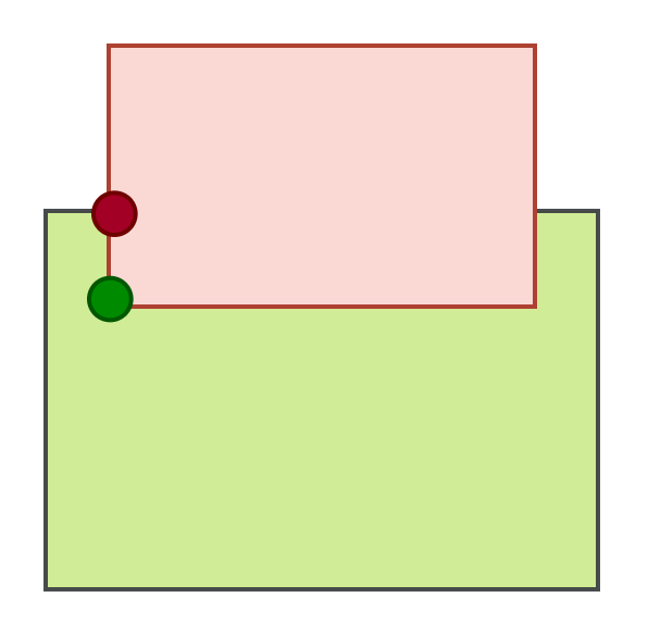
Wait, shouldn't this give us the same point every frame?
Yes. The issue with incremental manifolds arises after the collision detection step is completed, and a slight perturbation of the object is necessary. Various solutions exist for this, such as running collision detection on the points obtained in that round or manually rotating the objects until a complete manifold is obtained. This rotation causes a change in the value of the deepest penetration and the contact normal, resulting in a different output. 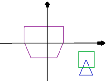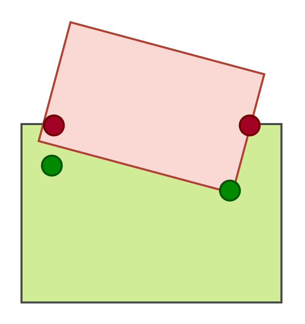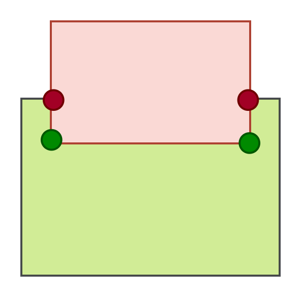To illustrate this, consider a simple 2D example. Note that the perturbation in actual physics simulations is much smaller.

Contact point(s)

• Book: Collision detection in interactive 3D environments by Gino van den Bergen
• You can get the full code from my Github repository: EPA

And with that we are finished with EPA! In the next (and last) article in this series we will be looking at another way to generate contact points.